Mich Talebzadeh

A Guide to Successful Big Data Implementation July 24, 2016

As a consultant I spend most of my time on a number of Big Data Projects (BDP). Big Data refers to the vast amount of Data being generated and stored, and the advanced analytics processes which are being developed to help make sense of this Big Data. Some of these projects are green fields and some are in advanced stage. Not surprisingly a number of these projects are kicked off without a definitive business use case and follow the trend in the Market, in layman’s term what I call Vogue of the Month.

As a consequence, a number of these projects fail and regrettably the proportion of this failure is greater than the other IT projects. In my opinion, by far insufficient scoping of the project has been responsible for the majority of BDP failures. In some cases, the goal post either changed too often or project objectives were not well defined in advance or too much was expected from the project.

There is another dimension to add to this. The technology landscape of Big Data is very fluid and in some cases relying on immature technology, much of which is open source with little use case (meaning used in production) has resulted in costly failures.

Like any other I.T. project if Big Data Project cannot deliver business value and was created as a purely technology concern and focus, then one should not be surprised for its lack of success.

Whilst there is a general agreement on the value of Big Data, a big data project should work under the same constraints that other IT projects work with well-defined objectives and roadmap.

A BDP by definition is riskier that the other established IT projects because of:

1. Immature technology stack in some cases
2. Lack of trained resources in Big Data to deliver that technology. Companies are still struggling to get adequate resources in.

So how do you make a Big Data Project a success? While how you manage your Big Data project can vary depending on your specific use case and your business space, there are a number of key steps to successfully implement a BDP and for the sake of brevity I have combined some together. These are as follows:

1. Your Business Use Case
2. The Project Plan and Scope
3. The Constraints and the Critical Success Factors
4. Assumptions
5. Reporting
6. Deliverables
7. Establish the Technical Requirements and Technology 
8. Create a Business Value Case

Your Business Use Case

Outline the tangible benefits that Big Data solution will bring. If you are a technical professional, you will need to:

• Outline what Big Data can do for the business concerned in terms that someone with business background can buy into it. In other words, how the business users are going to interact with the Big Data solution to achieve a specific business goal.
• Who are your business stakeholders and their roles? Business stakeholders normally have their agenda based on often other needs and these needs may create race conditions between stakeholders for their demands.
• Create if needed a Force Field Analysis of stakeholders who are in favor of changes proposed by Big Data and those who show little or no interest in embracing this change. From my experience people do not normally like change and they are content with status quo. You need to take them on board. This is part of the classic Critical Success Factor
• Prioritize Big Data use case taking into account different interests as discussed earlier
• What are the obstacles to getting there in terms of business and technology stack? Case in point, can a technology stack like Spark Streaming provide an adequate business solution for Algorithmic Trading in place of the propriety software?
• Manage the expectation. In some cases, Big Data may not be the answer to the problem and the solution may lie somewhere else.

I cannot emphasize enough the importance of a well-defined Business Use Case. You will need the Big Data goals outlined as clearly and as early as possible to avoid project failure.

The Project Plan and Scope

You need to define clear project plan and objectives here. Examples; to provide: Credit Risk needs, Insurance Risk Models, Fraud Detection, Real Time Data Analytics for a vendor’s tool, Sentiment Analysis and others

• Specify expected goals in measurable business terms. The goal here is a statement of specifics that quantify an objective.
• Identify all business criteria as precisely as you can determine.
• More often than not, you may need to phase the project in line with the available resources and absorption of Big Data Technology.
• Outline the need for Proof of Concept or Pilot Projects in advance.
• Dependency on the external consultants factored in if any.
• Create and maintain a project plan.

See also the Deliverables below

The Constraints and the Critical Success Factors

• Allocation of adequate time and resources by the Stakeholders Team in order for BDP to succeed
• Provision of adequate level of access to various resources including in-house staff, external consultants if any and Hardware such that an informed judgment at any part of the project can be made.
• Agreement on the timescales
• Resolution of all the technical and access matters.

Assumptions

BDP is normally a high profile assignment which may have long term consequences on the way the enterprise conducts its business. The following assumptions are made:

• Resources will be available from all departments at key points during the lifetime of this assignment. These include all resource types
• The Relevant Managers are required to make these resources available and committed to this assignment
• This assignment will address the point whether it is possible to create a satisfactory Big Data Solution for the enterprise needs. To this effect we expect A BDP to take a high profile.
• The commitment of the Senior Management to see this assignment through.

Reporting

As a consultant, I provide a comprehensive report upon the completion of the assignment. This report will form the bulk of the deliverables (see below). Additionally, a bi-weekly progress report needs to be provided to the stakeholders throughout the work undertaken. I find this adequate.

Deliverables

The deliverables have to be tightly coupled with the Project Scope such that BDP does not suffer from the Moving Target Syndrome so to speak. As a minimum:

• What is in scope in detail
• Equally import, what is not going to be delivered or out of scope
• If the project is phased what are the clear deliverables for each phase and the interfaces between these phases
• A comprehensive report highlighting the areas covered under the heading “Project Plan and Scope”
• The milestones that impact the deliverables
• The items that are on the critical path. For example, relying on a Big Data Vendor to deliver a given solution
• Show stoppers if any

Establishing the Technical Requirements and Technology Stack

This section is more important in case of Big Data compared to other more established technology stacks. These include stacks from the Ingestion Layer up to and including the Presentation Layer (I assume that the reader is familiar with these Big Data layers. Otherwise please see my other articles). In short how you are going to collect data and how you are going to present that data as a service

• The current tools available for Big Data Ingestion including the existing tools
• The existing architecture for interconnecting individual silos
• The volume of ETL and ELT involved
• The existence of a Master Data Model (MDM) if any
• External feeds etc.
• The usual three Vs of Big Data namely; Volume, Velocity and Variety
• These are shown in Figure 1 below

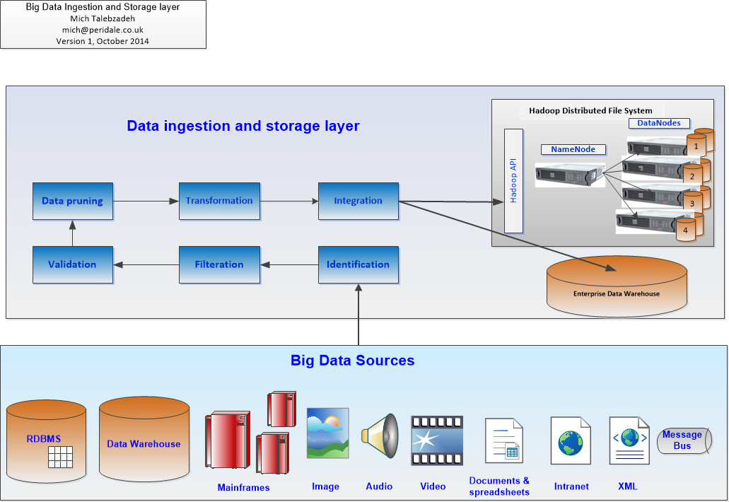
Figure 1: Big Data Ingestion and Storage Layer

Data in Motion versus Data at Rest. If Data in Motion is important, for example Real Time Fraud Detection (anything below 0.5 seconds), would it be useful to use some form of Data Fabric for a timely action and alert as shown in Figure 2 below:

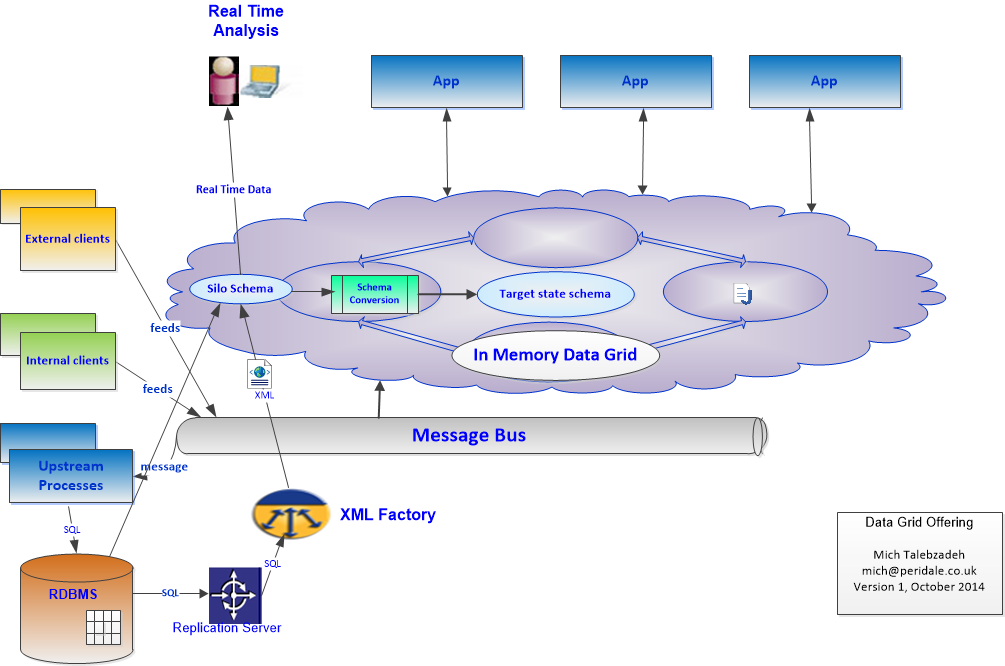
Figure 2: Data Grid Offering for Real Time Action

Your technical requirements will also have to cater for Big Data Analysis layer including the Analytics Engines and Model Management in order to provide business solutions as defined by the stakeholders as shown in Figure 3 below. For those interested in details please see my other articles here on Big Data.

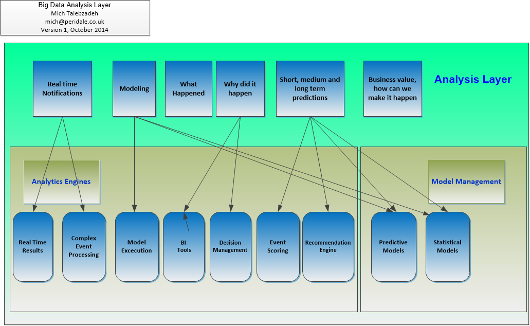
Figure 3: Big Data Analysis Layer

The Consumption Layer is the Client Facing Layer that has to satisfy the Stakeholders needs. This is a very important layer as it offers Data in various format as a Service to the Client. This is shown in Figure 4 below:

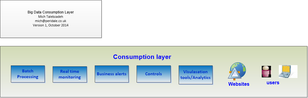
Figure 4: Big Data Consumption Layer

This is a layer that in which some investment is already been made and most stakeholders are familiar with this layer. In reality most medium and Large enterprises have already impressive proprietary  tools such as Oracle BI or Tableau for this purpose that hook to various Data Warehouses or Data Marts. From my experience a two-tier solution may work. This will allow the existing BI users to use the existing visualisation tools but crucially under the bonnet you may decide to move away from the proprietary Data Warehouse to Big Data. These considerations should be taken into account:

• The performance. Whether you keep using the existing Data Warehouse or Big Data storage layer such as HDFS, you should provide comparable performance
• Comparable Open Source tools. For example, you may deploy a simple Open Source tool like Apache Squirrel that allows SQL access to a variety of JDBC data sources including Big Data
• Consider taking advantage of in-memory offerings such as Apache Alluxio or the new kid in the block LLAP
•  Your technical users may want to delve into data above and beyond SQL type queries. In that case you may consider a notebook like Apache Zeppelin.

Create a Business Value Case 

Your Business Value Case needs to be in line with what the firm offers as its main line of business vis-à-vis deploying Big Data. In most cases this boils down to the tangible values that adding Big Data stack brings in. Very often this is not well established and very fluid in line of “let us see what we can get out of it for our business”. Your customers here are not IT stakeholders, but rather business stakeholders who are part of revenue generators and should use Big Data as insight for competitive advantage to make higher profits.

Think of it as this way. If Big Data Deployment is going to provide a favorable Return on Investment, you will need to quantify this one with a Cost/Benefit Analysis. A typical cost/benefit analysis should include the following:

Cost Assumptions

•  Working days in a Month = 20
• Uniform overall cost of resource per day. This varies from enterprise to enterprise but could be somewhere between £700 to £1200 per day.

Cost Calculation

• Upfront investment cost
• Implementation Cost over the period of the project
• Ongoing maintenance cost
• Licensing cost including Big Data vendor’s package and support
• Internal Cloud Storage Cost if any. Most Financial entities operate in this mode
• External Cloud Storage Cost if any. Small and Medium size companies may opt for Amazon S3 or Microsoft Azure
• Training cost for new technology
• New hardware cost
• Other costs

Benefits

• Faster and better decision making due to the availability of all resources in one place (Big Data Lake)
• Open source cost adjustment
• Sophisticated analytics can potentially improve decision-making process
• Avenues for new products and services that were not available before
• New information driven business model based on much better insight into the customers and competitors

Although some of the above points cannot not be converted into business values straight away, nonetheless they could be treated as a long term investment. Thus you have to consider the so called return on investment (ROI) value, in other words when you are going to see deploying Big Data is going to bring tangible profits.

Scalability

The business model evolves and so should your Big Data solution. You will need to build enough scalability to the Big Data Solution to allow painless expansion to support future expansion. This is no different from the classic I.T. solutions

Simplicity

Since my student days I have believed that there is a well-established scientific axiom namely “Simple is beautiful”. If a product offers simple solution for complicated problems, then it must be a well-designed product by definition. Like any other software build, there are two ways of constructing a Big Data solution. One way is to make it simple or simple enough that there are obviously no deficiencies, and the other way is to make it so complicated that there are no obvious deficiencies. The first method is far more difficult to achieve due to the current state of Big Data landscape which is crowded by often confusing and conflicting offerings.

Thus it is important to keep the technology stack as simple and robust as possible. For example, supporting two overlapping products at the same is a recipe for fragmentation and resource wastage.

Conformation to Open Standards

Your choice of open source product has to be based on sound decision taking into account:

•  Enterprise Readiness. Simply put whether the product is ready for production deployment
• The support within the community.
• The stability of the product
• The ease of maintainability
• Whether the product is supported by a Big Data vendor
• The potential risk associated with deploying a promising but little known product
• The level of in-house expertise in supporting and acting quickly if there is an issue with any component of Big Data

Summary

I trust that I have provided some useful information here. Like anything else there is no hard and fast rule on how to implement a Big Data Project. Some will find to use some Structured method to implement it or other mortals like myself prefer a heuristic model based on one’s existing experience and knowledge. As ever your mileage varies.

Disclaimer: Great care has been taken to make sure that the technical information presented in this paper is accurate, but any and all responsibility for any loss, damage or destruction of data or any other property which may arise from relying on its content is explicitly disclaimed. The author will in no case be liable for any monetary damages arising from such loss, damage or destruction

Presentation in London: Query Engines for Hive: MR, Spark, Tez with LLAP – Considerations! July 7, 2016

I will be presenting on the topic of “‘Query Engines for Hive: MR, Spark, Tez with LLAP – Considerations!” in Future of Data: London

Details

Organized by: Hortonworks

Date: Wednesday, July 20, 2016, 6:00 PM to 8:30 PM 

Place: London

Location:La Tasca West India Docks Road E14

If you are interested please register here

Looking forward to seeing those who can make it to have an interesting discussion and leverage your experience.

Abstract

Apache Hive has established itself to be the Data Warehouse of choice on Hadoop for storing data on HDFS and compatible file systems. Hive has been using the standard MapReduce as its execution engine for a while. Newer release of Hive allow Apache Spark or Apache Tez together with LLAP to be used as its query engines as well. With the ability of Hive to deploy these different performant execution engines, it is important to understand the benefits and limitations that each engine brings in coming to an informed decision in deploying them. Mich will discuss how to set up Spark as execution engine for Hive and will present some interesting results. In addition, the presentation has now been extended to cover the deployment of Tez together with LLAP as a hybrid execution engine for Hive with equally interesting findings.

The proceeding are available here

A Roadmap for Careers in Big Data July 2, 2016

We are pleased to inform you that Hortonworks in association with Mich Talebzadeh and Radley James have organized this forthcoming presentation in London on Wednesday 17th August 18:00 BST, on Roadmap for Careers in Big Data.

Registration are open now. You can register here.

Whether you are an Architect, a DBA, a Developer or Analyst you will hopefully benefit from such presentation. By the end of the talk you will be shown the roadmap to Big Data, the buzzwords and the emerging new products expanding at amazing pace. You will gain a better understanding of Big Data to add to your existing skills. You will know how to relate your existing (often relational) knowledge to Big Data and build upon it. If you are contemplating moving to Big Data or simply would like to broaden your horizon, this presentation is a must for you. We have the experts to help you.

Mich Talebzadeh will start outlining his journey from the relational world to Big Data followed by Hortonworks experts who will delve deeper into Big Data world and present practical steps that you can take to be more proficient in Big Data. There will be a road map for both on-line and classroom training provided by Hortonworks up to the certification and expert level.

Finally, the specialist recruitment agency Radley James will present their expertise in helping you out in your quest for careers in Big Data and their extensive contacts in many market sectors.

Let us get together for some beers and pizza at Hortonworks’ London office to learn more about this exciting new world. As the saying goes; learn more, earn more.

A word about the Organizers

Hortonworks is a leading innovator in the industry, creating, distributing and supporting enterprise-ready open data platforms and modern data applications. Our mission is to manage the world’s data. Founded in 2011, we have a single-minded focus on driving innovation in open source communities such as Apache Hadoop, NiFi, and Spark. We along with our 1600+ partners provide the expertise, training and services that allow our customers to unlock transformational value for their organizations across any line of business. Our connected data platforms power modern data applications that deliver actionable intelligence from all data: data-in-motion and data-at-rest. We are Powering the Future of Data. More than a third of Big Data committers come from Hortonworks.

Mich Talebzadeh is an award winning technologist and architect who has worked with data and database management systems since his student days at the Imperial College of Science and Technology, University of London, where he obtained his PhD in Particle Physics. He specializes in the strategic use of Big Data ecosystem, RDBMS, IMDB and CEP. Mich is the co-author of “Sybase Transact SQL Programming Guidelines and Best Practices”, author of “A Practitioner’s Guide to Upgrading to Sybase ASE 15” and the author of the forthcoming book “Complex Event Processing in Heterogeneous Environments” and numerous articles.  Mich is also a contributor to Big Data User Groups Like Apache Spark and Apache Hive.

Radley James is one of the most successful Finance and Technology Recruitment agencies in the world today. Boasting a dynamic team with a breadth of relevant experience – we can provide you with outstanding talent in Big Data, Project Management, Cyber Security, Digital, Software Development and Quantitative Research across many diverse sectors such as Investment Banking, Hedge Fund companies, Prop Trading houses, Consultancy, Retail, Corporate Banks and Insurance. We have now a newly established division totally dedicated to Big Data.

My Newer Posts on Big Data January 15, 2016

My newer posts on Big data are currently as follows:

• A Roadmap for Careers in Big Data, June 2016
• A Possible Next Career Move for Relational DBAs, June 2016
• A Winning Strategy – Running Apache Hive on Spark Execution Engine (part 1), May 2016
• Apache Hive Data Warehouse and a proposal to improve Hive external indexes, May 2016
• Big Data And the Myth of Hadoop Demise Apr 15, 2016
• Apache Hive 2 is now Released Feb 18, 2016
• The old SQL, the Jewel in the Crown of RDBMS and now Big Data Feb 16, 2016
• Hive on Spark Engine Versus Spark Using Hive Metastore Feb 7 2016
• ORC Columnar File and Storage Index in Hive, Feb 2 2016
• ETL or ELT and the Use Case, Jan 5 2016
• DIY in the Festive Season. How to install and configure Big Data Hadoop in an hour or so, Dec 28 2015
• Apache Hive, Engine processing in memory or on disk, Dec 16 2015
• Getting ready for IFRS 9 and the Big Data Role, Dec 12 2015
• Big Data in Action for those familiar with Relational Databases and SQL, Dec 9 2015
• Technical Architect and the challenge of Big Data Architecture, Nov 30 2015
• Data Grid and Big Data Architecture with Hadoop and Hive, Nov 26 2015
• An Architecture for Real Time Analytics of Big Data , Nov 21 2015

They are all in my LinkedIn profile here

How to install and configure Big Data Hadoop in an hour or so (does not include your coffee break) May 25, 2015

Pre-requisites

1) Have a Linux host running a respectable flavor of Linux. Mine is RHES 5.2 64-bit. I also have another host using RHES 5.2, 32-bit which also has Hadoop installed on it.
2) Basic familiarity with Linux commands
3) Oracle Java Development Kit (JDK) 1.5 or higher
4) Configuring SSH access
5) Setting ulimit (optional)

Creating group and user on Linux

Log in as root to your Linux host and create a group called hadoop2 and user hduser2. Note since I already have goup/user hadoop/hduser, I decided for the sake of this demo to create new ones on the same host

root@rhes564 ~]# groupadd hadoop2
[root@rhes564 ~]# useradd -G hadoop2 hduser2

You will see that a home directory for user hduser2 called /home/hduser2 is created.

ls -ltr /home
drwx------ 3 hduser2 hduser2 4096 May 24 09:30 hduser2
[root@rhes564 home]# su - hduser2
[hduser2@rhes564 ~]$ pwd
/home/hduser2

You can edit [root@rhes564 home]# vi /etc/passwd file to change the default shell for hduser2
I changed it to korn shell

hduser2:x:1013:1015::/home/hduser2:/bin/ksh

Now set the password for hduser2 as below

[root@rhes564 home]# passwd hduser2
Changing password for user hduser2.
New UNIX password:
Retype new UNIX password:
passwd: all authentication tokens updated successfully.

## log in as hduser2

su - hduser2
Password:
 id
uid=1013(hduser2) gid=1015(hduser2) groups=1015(hduser2)

So far so good. We have set up a new user hduser2 belonging to the group hadoop2. Make sure that the ownership is correct. As root do

</pre>
[root@rhes564 ~]# chown -R hduser2:hadoop2 /home/hduser2

Now you need to set up your shells. The Korn shell uses two startup files, the .profile and the .kshrc. The .profile is read once, by your login ksh, while the .kshrc is read by each new ksh.
I put all my environment in .kshrc file.

Remember most of this Big Data is developed in Java. so you will need an up-to-date version of JDK installed. The details for me are as follows:

$ which java
/usr/bin/java
$ java -version
java version "1.7.0_21"
Java(TM) SE Runtime Environment (build 1.7.0_21-b11)
Java HotSpot(TM) 64-Bit Server VM (build 23.21-b01, mixed mode)

My sample .profile is as follows:

$ cat .profile
stty erase ^?
PATH=/bin:/sbin:/usr/bin:/usr/sbin:/usr/local/bin:/usr/local/sbin:/usr/bin/X11:/usr/X11R6/bin:/root/bin
unset LANG
export ENV=~/.kshrc
. ./.kshrc

I will come to this later.

Setting up ssh

Hadoop relies on ssh to access different nodes and loop back to itself.  Although this is a single node setup, you will still need to set up ssh.  It is pretty straight forward and you happen to be a a DBA or developer, you have already done this many times for oracle or sybase accounts.

ssh-keygen -t rsa -P ""
Generating public/private rsa key pair.
Enter file in which to save the key (/home/hduser2/.ssh/id_rsa):
Created directory '/home/hduser2/.ssh'.
Your identification has been saved in /home/hduser2/.ssh/id_rsa.
Your public key has been saved in /home/hduser2/.ssh/id_rsa.pub.
The key fingerprint is:
97:af:a3:18:f8:30:74:3b:73:53:07:4d:16:e7:1b:8a hduser2@rhes564

Enable SSH access to your local machine with this newly created key.

cat $HOME/.ssh/id_rsa.pub >> $HOME/.ssh/authorized_keys

Now test ssh by connecting to localhost for user hduser2 and see if it works. It will also add to file known_hosts under directory $HOME/.ssh

ssh localhost
The authenticity of host 'localhost (127.0.0.1)' can't be established.
RSA key fingerprint is 21:75:c2:da:01:68:c4:ef:23:7b:d2:ac:e4:ef:06:02.
Are you sure you want to continue connecting (yes/no)? yes
Warning: Permanently added 'localhost' (RSA) to the list of known hosts.
Address 127.0.0.1 maps to rhes564, but this does not map back to the address - POSSIBLE BREAK-IN ATTEMPT!

This should work. Otherwise Google for ssh and use ssh in debug mode by typing ssh -vv localhost to debug the error

Increasing ulimit parameter for user hduser2

You may find later that you will require file descriptor value higher than the default value od 1024. As root edit the file etc/security/limits.conf and add the following lines to the bottom

hduser2 soft nofile 4096
hduser2 hard nofile 63536

Reboot host for this to take place. You will need to set it in your shell startup file for hduser2 as well

ulimit -n 63536

Installing Hadoop

You can download Hadoop from Apache Hadoop site from here. At the time of writing these notes (May 2015), the most recent release was release 2.6.0. Download the binary zipped file. It is around 200MB as shown below:

-rw-r--r-- 1 hduser2 hadoop2 210343364 May 24 11:07 hadoop-2.7.0.tar.gz

Unzip and untar the file. It will create a directory called hadoop-2.7.0 as below

drwxr-xr-x 9 hduser2 hadoop2 4096 Apr 10 19:51 hadoop-2.7.0

Now you need to setup your environment variables in your shell routine. Mine is .kshrc

#HADOOP VARIABLES START
export JAVA_HOME=/usr/java/latest
export HADOOP_HOME=${HOME}/hadoop-2.7.0
export PATH=$PATH:$HADOOP_HOME/bin
export PATH=$PATH:$HADOOP_HOME/sbin
export HADOOP_MAPRED_HOME=$HADOOP_HOME
export HADOOP_COMMON_HOME=$HADOOP_HOME
export HADOOP_HDFS_HOME=$HADOOP_HOME
export YARN_HOME=$HADOOP_HOME
export HADOOP_COMMON_LIB_NATIVE_DIR=$HADOOP_HOME/lib/native
export HADOOP_OPTS="-Djava.library.path=$HADOOP_HOME/lib"
#HADOOP VARIABLES END
export HADOOP_CLIENT_OPTS="-Xmx2g"
unset CLASSPATH
CLASSPATH=.:$HADOOP_HOME/share/hadoop/common/hadoop-common-2.7.0-tests.jar:$HADOOP_HOME/share/hadoop/common/hadoop-common-2.7.0.jar:hadoop-nfs-2.7.0.jar:$HIVE_HOME/conf
export CLASSPATH
ulimit -n 63536

The next step is to look at the directory tree for hadoop.

hduser2@rhes564::/home/hduser2> cd $HADOOP_HOME
hduser2@rhes564::/home/hduser2/hadoop-2.7.0> ls -ltr
total 52
drwxr-xr-x 4 hduser2 hadoop2 4096 Apr 10 19:51 share
drwxr-xr-x 2 hduser2 hadoop2 4096 Apr 10 19:51 libexec
drwxr-xr-x 3 hduser2 hadoop2 4096 Apr 10 19:51 lib
drwxr-xr-x 2 hduser2 hadoop2 4096 Apr 10 19:51 include
drwxr-xr-x 3 hduser2 hadoop2 4096 Apr 10 19:51 etc
drwxr-xr-x 2 hduser2 hadoop2 4096 Apr 10 19:51 bin
-rw-r--r-- 1 hduser2 hadoop2 1366 Apr 10 19:51 README.txt
-rw-r--r-- 1 hduser2 hadoop2 101 Apr 10 19:51 NOTICE.txt
-rw-r--r-- 1 hduser2 hadoop2 15429 Apr 10 19:51 LICENSE.txt
drwxr-xr-x 2 hduser2 hadoop2 4096 May 24 13:02 sbin

Note that unlike usual installation there is no conf directory here. Older versions of Hadoop had conf directory. This has now been replaced with etc directory. Below etc there is sub-directory called hadoop that has all the configuration files.

<pre>cd $HADOOP_HOME/etc/hadoop]
<pre> ls -ltr
total 152
-rw-r--r-- 1 hduser2 hadoop2 690 Apr 10 19:51 yarn-site.xml
-rw-r--r-- 1 hduser2 hadoop2 4567 Apr 10 19:51 yarn-env.sh
-rw-r--r-- 1 hduser2 hadoop2 2250 Apr 10 19:51 yarn-env.cmd
-rw-r--r-- 1 hduser2 hadoop2 2268 Apr 10 19:51 ssl-server.xml.example
-rw-r--r-- 1 hduser2 hadoop2 2316 Apr 10 19:51 ssl-client.xml.example
-rw-r--r-- 1 hduser2 hadoop2 10 Apr 10 19:51 slaves
-rw-r--r-- 1 hduser2 hadoop2 758 Apr 10 19:51 mapred-site.xml.template
-rw-r--r-- 1 hduser2 hadoop2 4113 Apr 10 19:51 mapred-queues.xml.template
-rw-r--r-- 1 hduser2 hadoop2 1383 Apr 10 19:51 mapred-env.sh
-rw-r--r-- 1 hduser2 hadoop2 951 Apr 10 19:51 mapred-env.cmd
-rw-r--r-- 1 hduser2 hadoop2 11237 Apr 10 19:51 log4j.properties
-rw-r--r-- 1 hduser2 hadoop2 5511 Apr 10 19:51 kms-site.xml
-rw-r--r-- 1 hduser2 hadoop2 1631 Apr 10 19:51 kms-log4j.properties
-rw-r--r-- 1 hduser2 hadoop2 1527 Apr 10 19:51 kms-env.sh
-rw-r--r-- 1 hduser2 hadoop2 3518 Apr 10 19:51 kms-acls.xml
-rw-r--r-- 1 hduser2 hadoop2 620 Apr 10 19:51 httpfs-site.xml
-rw-r--r-- 1 hduser2 hadoop2 21 Apr 10 19:51 httpfs-signature.secret
-rw-r--r-- 1 hduser2 hadoop2 1657 Apr 10 19:51 httpfs-log4j.properties
-rw-r--r-- 1 hduser2 hadoop2 1449 Apr 10 19:51 httpfs-env.sh
-rw-r--r-- 1 hduser2 hadoop2 775 Apr 10 19:51 hdfs-site.xml
-rw-r--r-- 1 hduser2 hadoop2 9683 Apr 10 19:51 hadoop-policy.xml
-rw-r--r-- 1 hduser2 hadoop2 2598 Apr 10 19:51 hadoop-metrics2.properties
-rw-r--r-- 1 hduser2 hadoop2 2490 Apr 10 19:51 hadoop-metrics.properties
-rw-r--r-- 1 hduser2 hadoop2 4224 Apr 10 19:51 hadoop-env.sh
-rw-r--r-- 1 hduser2 hadoop2 3670 Apr 10 19:51 hadoop-env.cmd
-rw-r--r-- 1 hduser2 hadoop2 774 Apr 10 19:51 core-site.xml
-rw-r--r-- 1 hduser2 hadoop2 318 Apr 10 19:51 container-executor.cfg
-rw-r--r-- 1 hduser2 hadoop2 1335 Apr 10 19:51 configuration.xsl
-rw-r--r-- 1 hduser2 hadoop2 4436 Apr 10 19:51 capacity-scheduler.xml

Configuring Hadoop

The important configuration files are listed below. They are either shell files; *.sh or xml configuration files *.xml. The important ones are explained below

hadoop-env.sh

Edit file hadoop-env.sh and set JAVA_HOME explicitely

The java implementation to use.
export JAVA_HOME=/usr/java/latest

This will work as long as ${JAVA_HOME} is set up in your start-up shell.

XML files below work on specifying property. To override a default value for a property, specify the new value within the tags, using the following format:

<property>
   <name> </name>
   <value> </value>
   <description> </description>
</property>

core-site.xml

The only parameter I have put here is fs.default.name. you need a URI whose classscheme and authority determines the FileSystem implementation. The uri’s authority is used to determine the host, port, etc. for a filesystem.

<configuration>
<property>
<name>fs.default.name</name>
<value>hdfs://rhes564:19000</value>
</property>
</configuration>

So in my case I have the host as my host rhes564, and the port as 9000. Note that 9000 will be the port hadoop is running on. By default it is localhost:9000.

mapred-site.xml

MapReduce Engine runs on Hadoop. MapReduce configuration options are stored in mapred-site.xml file. This file contains configuration information that overrides the default values for MapReduce parameters.

Copy mapred-site.xml.template to mapred-site.xml. Edit this file and add the following lines:

<configuration>
<property>
 <name>mapreduce.framework.name</name>
 <value>yarn</value>
 <description> Execution framework set to Hadoop YARN </description>
</property>

<property>
 <name>mapreduce.job.tracker</name>
 <value>rhes564:54312</value>
 <description> The URL to track mapreduce jobs </description>
</property>

<property>
 <name>mapreduce.job.tracker.reserved.physicalmemory.mb</name>
 <value>1024</value>
 <description> The physical memory allocated for each job </description>
</property>

<property>
 <name>mapreduce.map.memory.mb</name>
 <value>2048</value>
 <description> mapreduce.map.memory.mb is the upper memory limit that Hadoop allows to be allocated to a mapper, in MB. </description>
</property>

<property>
 <name>mapreduce.reduce.memory.mb</name>
 <value>2048</value>
 <description> Larger resource limit for reduces </description>
</property>

<property>
 <name>mapreduce.map.java.opts</name>
 <value>-Xmx3072m</value>
 <description> Larger heap-size for child jvms of maps </description>
</property>

<property>
 <name>mapreduce.reduce.java.opts</name>
 <value>-Xmx6144m</value>
 <description> Larger heap-size for child jvms of reduces </description>
</property>

<property>
 <name>yarn.app.mapreduce.am.resource.mb</name>
 <value>400</value>
 <description> specifies "The amount of memory the MR AppMaster needs </description>
</property>
</configuration>

hdfs-site.xml

One of the most important configuration files. It stores configuration settings with regard to Hadoop HDFS NameNode and DataNode among other things . I have already discussed these two somewhere else. You will need to find reasonable space where you want HDFS data to be stored.

<configuration>
<property>
<name>dfs.replication</name>
<value>1</value>
<description> This set the number of replicates. For single node it is 1 </description>
</property>

<property>
<name>dfs.namenode.name.dir</name>
<value>file:/data4/hadoop/hadoop_store/hdfs/namenode</value>
<description> This is where HDFS metadata is stored </description>
</property>

<property>
<name>dfs.datanode.data.dir</name>
<value>file:/data4/hadoop/hadoop_store/hdfs/datanode</value>
<description> This is where HDFS data is stored </description>
</property>

<property>
<name>dfs.block.size</name>
<value>134217728</value>
<description> This is the default block size. It is set to 128*1024*1024 bytes or 128 MB </description>
</property>
</configuration>

yarn-site.xml

This file provides configuration parameters for resource manager YARN (Yet Another Resource Manager).

<configuration>
 <property>
 <name>yarn.nodemanager.aux-services</name>
 <value>mapreduce_shuffle</value>
 </property>
<property>
 <name>yarn.nodemanager.aux-services.mapreduce.shuffle.class</name>
 <value>org.apache.hadoop.mapred.ShuffleHandler</value>
</property>
<property>
 <name>yarn.nodemanager.vmem-check-enabled</name>
 <value>false</value>
</property>
</configuration>

Formatting Hadoop Distributed File System (HDFS)

Before starting Hadoop we need to format the underlying file system. This is required when you set up Hadoop first time. Think of it as formatting your drive. You need to shutdown Hadoop whenever you format HDFS. Remember if you format it again you will lose all data! To perform the format you use the following command:

hdfs namenode -format

If you have set up your path in your start up (you have it), then hdfs will be on the path. Otherwise it is under $HADOOP_HOME/bin/hdfs. This is the ouput from the command

<pre>hdfs namenode -format
15/05/25 19:27:20 INFO namenode.NameNode: STARTUP_MSG:
/************************************************************
STARTUP_MSG: Starting NameNode
STARTUP_MSG: host = rhes564/50.140.197.217
STARTUP_MSG: args = [-format]
STARTUP_MSG: version = 2.7.0

----

15/05/25 19:27:21 INFO namenode.FSNamesystem: dfs.namenode.safemode.threshold-pct = 0.9990000128746033
15/05/25 19:27:21 INFO namenode.FSNamesystem: dfs.namenode.safemode.min.datanodes = 0
15/05/25 19:27:21 INFO namenode.FSNamesystem: dfs.namenode.safemode.extension = 30000
15/05/25 19:27:21 INFO metrics.TopMetrics: NNTop conf: dfs.namenode.top.window.num.buckets = 10
15/05/25 19:27:21 INFO metrics.TopMetrics: NNTop conf: dfs.namenode.top.num.users = 10
15/05/25 19:27:21 INFO metrics.TopMetrics: NNTop conf: dfs.namenode.top.windows.minutes = 1,5,25
15/05/25 19:27:21 INFO namenode.FSNamesystem: Retry cache on namenode is enabled
15/05/25 19:27:21 INFO namenode.FSNamesystem: Retry cache will use 0.03 of total heap and retry cache entry expiry time is 600000 millis
15/05/25 19:27:21 INFO util.GSet: Computing capacity for map NameNodeRetryCache
15/05/25 19:27:21 INFO util.GSet: VM type = 64-bit
15/05/25 19:27:21 INFO util.GSet: 0.029999999329447746% max memory 888.9 MB = 273.1 KB
15/05/25 19:27:21 INFO util.GSet: capacity = 2^15 = 32768 entries
Re-format filesystem in Storage Directory /data4/hadoop/hadoop_store/hdfs/namenode ? (Y or N) y
15/05/25 19:28:40 INFO namenode.FSImage: Allocated new BlockPoolId: BP-959407252-50.140.197.217-1432578520863
15/05/25 19:28:40 INFO common.Storage: Storage directory /data4/hadoop/hadoop_store/hdfs/namenode has been successfully formatted.
15/05/25 19:28:41 INFO namenode.NNStorageRetentionManager: Going to retain 1 images with txid >= 0
15/05/25 19:28:41 INFO util.ExitUtil: Exiting with status 0
15/05/25 19:28:41 INFO namenode.NameNode: SHUTDOWN_MSG:
/************************************************************
SHUTDOWN_MSG: Shutting down NameNode at rhes564/50.140.197.217
************************************************************/

If you repeat the command again, you will get a message

Re-format filesystem in Storage Directory /data4/hadoop/hadoop_store/hdfs/namenode ? (Y or N)

If you confirm it, it will be reformatted.

Putting the show on the road, Starting Hadoop

Go ahead and start hadoop daeomons

start-dfs.sh

15/05/25 19:51:28 WARN util.NativeCodeLoader: Unable to load native-hadoop library for your platform... using builtin-java classes where applicable
Starting namenodes on [rhes564]
rhes564: starting namenode, logging to /home/hduser2/hadoop-2.7.0/logs/hadoop-hduser2-namenode-rhes564.out
localhost: Address 127.0.0.1 maps to rhes564, but this does not map back to the address - POSSIBLE BREAK-IN ATTEMPT!
localhost: starting datanode, logging to /home/hduser2/hadoop-2.7.0/logs/hadoop-hduser2-datanode-rhes564.out
Starting secondary namenodes [0.0.0.0]
0.0.0.0: Address 127.0.0.1 maps to rhes564, but this does not map back to the address - POSSIBLE BREAK-IN ATTEMPT!
0.0.0.0: starting secondarynamenode, logging to /home/hduser2/hadoop-2.7.0/logs/hadoop-hduser2-secondarynamenode-rhes564.out
15/05/25 19:51:43 WARN util.NativeCodeLoader: Unable to load native-hadoop library for your platform... using builtin-java classes where applicable

If you get an error JAVA_HOME not set, make sure that you have modified and set JAVA_HOME in hadoop-env.sh. Ignore WARNs

To check that your Hadoop started on port 19000 (as we set in core-site.xml file), do the following

netstat -plten|grep java

(Not all processes could be identified, non-owned process info
 will not be shown, you would have to be root to see it all.)
tcp 0 0 50.140.197.217:19000 0.0.0.0:* LISTEN 1013 31595 12540/java

There it is running under process 12540. You can see it in full glory

ps -efww | grep 12540
hduser2 12540 1 0 19:51 ? 00:00:04 /usr/java/latest/bin/java -Dproc_namenode -Xmx1000m -Djava.net.preferIPv4Stack=true -Dhadoop.log.dir=/home/hduser2/hadoop-2.7.0/logs -Dhadoop.log.file=hadoop.log -Dhadoop.home.dir= -Dhadoop.id.str=hduser2 -Dhadoop.root.logger=INFO,console -Djava.library.path= -Dhadoop.policy.file=hadoop-policy.xml -Djava.net.preferIPv4Stack=true -Djava.net.preferIPv4Stack=true -Djava.net.preferIPv4Stack=true -Dhadoop.log.dir=/home/hduser2/hadoop-2.7.0/logs -Dhadoop.log.file=hadoop-hduser2-namenode-rhes564.log -Dhadoop.home.dir=/home/hduser2/hadoop-2.7.0 -Dhadoop.id.str=hduser2 -Dhadoop.root.logger=INFO,RFA -Djava.library.path=/home/hduser2/hadoop-2.7.0/lib/native -Dhadoop.policy.file=hadoop-policy.xml -Djava.net.preferIPv4Stack=true -Dhadoop.security.logger=INFO,RFAS -Dhdfs.audit.logger=INFO,NullAppender -Dhadoop.security.logger=INFO,RFAS -Dhdfs.audit.logger=INFO,NullAppender -Dhadoop.security.logger=INFO,RFAS -Dhdfs.audit.logger=INFO,NullAppender -Dhadoop.security.logger=INFO,RFAS org.apache.hadoop.hdfs.server.namenode.NameNode

You can start other processes as below

yarn-daemon.sh start resourcemanager

starting resourcemanager, logging to /home/hduser2/hadoop-2.7.0/logs/yarn-hduser2-resourcemanager-rhes564.out

yarn-daemon.sh start nodemanager

starting nodemanager, logging to /home/hduser2/hadoop-2.7.0/logs/yarn-hduser2-nodemanager-rhes564.out

mr-jobhistory-daemon.sh start historyserver

starting historyserver, logging to /home/hduser2/hadoop-2.7.0/logs/mapred-hduser2-historyserver-rhes564.out

If all goes well (and it should), you will hopefully get no error messages. Just to check all processes are running OK, do as follows at the command line using Jps. Jps (Java Processes Status) should come back with the list. It is part of JDK and is under $JAVA_HOME/bin. It is equivalent to ps command. It lists all java Processes of a user.

jps

<pre>13510 JobHistoryServer
12540 NameNode
12839 SecondaryNameNode
13127 ResourceManager
13374 NodeManager
13629 Jps
12637 DataNode

Shutting down Hadoop

stop-dfs.sh

15/05/25 20:28:16 WARN util.NativeCodeLoader: Unable to load native-hadoop library for your platform... using builtin-java classes where applicable
Stopping namenodes on [rhes564]
rhes564: stopping namenode
localhost: Address 127.0.0.1 maps to rhes564, but this does not map back to the address - POSSIBLE BREAK-IN ATTEMPT!
localhost: stopping datanode
Stopping secondary namenodes [0.0.0.0]
0.0.0.0: Address 127.0.0.1 maps to rhes564, but this does not map back to the address - POSSIBLE BREAK-IN ATTEMPT!
0.0.0.0: stopping secondarynamenode
15/05/25 20:28:34 WARN util.NativeCodeLoader: Unable to load native-hadoop library for your platform... using builtin-java classes where applicable

yarn-daemon.sh stop resourcemanager

stopping resourcemanager

yarn-daemon.sh stop nodemanager

stopping nodemanager

mr-jobhistory-daemon.sh stop historyserver

stopping historyserver

Web Interfaces

Once the Hadoop is up and running, you can use the following web interfaces for various components:

Daemon		        Web Interface		        Notes
NameNode		http://host:port/		Default HTTP port is 50070.
MapReduce Jobs	        http://host:port/        	Default HTTP port is 8088.

Big Data in Action for those familiar with relational databases and SQL, part 2 May 16, 2015

What is schema on write

Most people who deal with relational databases are familiar with Schema on Write. In an RDBMS there are schemas/databases, tables, other objects and relationships. Every table has a well defined structure with column names, data type and column level constraint among others. A developer needs to know the schema beforehand before he/she can insert a row into that table. One cannot insert a varchar value into an integer column. Even adding a column to a table will require planning and code changes. If you are replicating the table then the replication definition will have to be modified as well to reflect that additional column, otherwise data will be out of sync at the replicate. So in short you need to know the schema at time of writing to the database. This is “schema on write” that is, the schema is applied when the data is being written to the database.

What is schema on read

In contrast to “schema on write”, the “schema on read” is applied as the data is being read off of the storage. The idea is that we decide what the schema is when we analyze the data as opposed to when we write the data. In other words with the massive heap that we have stored in Hadoop, we decide what to take out and analyze (and make sense out of it). So schema on read means write your data first, figure out what it is later. Schema on write means figure out what your data is first, then write it after.

Moving on

So there are a number of points to note. In schema on write we sort out and clean data first. In other words we do Extract, Transform and Load (ETL) before storing data to the source table. In schema on read, we add to data as is and then decide how to do ETL, slice and dice the data later. So when we hear that a very large amount of data is loaded daily to Hadoop, that basically means that the base table is augmented with new inserts, new updates and new deletes. OK. I am sure you will be happy with new inserts. That is the data inserted into the source table in Oracle or Sybase. How about updates or deletes? Unlike Oracle or Sybase we don’t go and update or delete rows in place. In Hive the correct mechanism (that you need to devise) is that every updated or deleted row will be a new row/entry added to Hive table with the correct flag and timestamp to identify the nature of DML.

There are three record types added to Hive table in any time interval. They follow the general CRUD (create, read, Update, Delete) rules. Within Entity Life History every relational table will have one insert type for a given Primary Key (PK), one delete for the same PK and many updates for the same PK. So we will end up within a day with new records, new updates and deleted records. Crucially a row in theory may be updated infinite times within a time period but what matters is the most “recent” update as far as a relational table is concerned. In contrast, the said table in Hive will be a running total of original direct loads from Oracle or Sybase table plus all new operations (CRUD) as well. For those familiar with replication, you sync the replicate once and let replication take care of new inserts, updates and deletes thereafter. The crucial point being that rather than row updates or deletes, you append the updated row or deleted row as a new row to Hive table. Well that is the art of Big Data so to speak. I will come back how to do the ETL in Hive as well.

On the face of it this looks a bit messy. However, we have to take into account the enormous opportunities that this technique will offer in terms of periodic reports of what happened, projections, opportunities etc. As a simple example, if I was audit, I could go and look at when a trade was created, how often it was updated, when it was settled and finally purged (deleted). The source Oracle or Sybase table may have deleted the record, however, the record will always be accessible in Hive. In other words as mentioned before Hive offers economies of cheap storage plus schema on read.

Cheap storage means that in theory you can use any storage without the need to use RAID or SAN. Well not exactly rushing to PC World to buy yourself some extra hard drives :). These can be JBOD. The name JBOD, just a bunch of disks refers to an architecture involving multiple hard drives much like commodity hardware using them as independent hard drives, or as a combined (spanned) single logical volume with no actual RAID functionality. This makes sense as HDFS takes the role of redundancy by having multiple copies of the data on different disks within HDFS cluster. Having said that I have seen Big Data application installed on SAN disks which sort of defeats the purpose of having redundant data within the cluster.

Setting up Hive

The easiest way to install Hive is to create it under Hadoop account in Linux. For example my Hadoop set up runs under user hduser:hadoop

id
uid=1009(hduser) gid=1010(hadoop) groups=1010(hadoop)

The recommendation is that you install Hive under /usr/lib/ directory. Briefly use your root account to create directory /usr/lib/hive and unzip and untar hive binaries under that directory. Change the ownership of directory and files to hduser:hadoop.

You need to modify your start up shell to include the following:

 
export HIVE_HOME=/usr/lib/hive
export PATH=/$HIVE_HOME/bin:$PATH

All Big Data components like Hadoop, Hive etc come with various configuration files. In Hive this file is called $HIVE_HOME/bin/hive-core.xml. That is akin to the configuration file SPFILE.ora in Oracle or the cfg file in Sybase ASE. You configure Hive using this xml file.

Let us understand the directory tree under Hive.

hduser@rhes564::/usr/lib/hive> ls -ltr
total 396
drwxr-xr-x 4 hduser hadoop 4096 Mar 7 22:38 examples
drwxr-xr-x 7 hduser hadoop 4096 Mar 7 22:38 hcatalog
drwxr-xr-x 3 hduser hadoop 4096 Mar 7 22:38 scripts
-rw-r--r-- 1 hduser hadoop 340611 Mar 7 22:38 RELEASE_NOTES.txt
-rw-r--r-- 1 hduser hadoop 4048 Mar 7 22:38 README.txt
-rw-r--r-- 1 hduser hadoop 277 Mar 7 22:38 NOTICE
-rw-r--r-- 1 hduser hadoop 23828 Mar 7 22:38 LICENSE
drwxr-xr-x 5 hduser hadoop 4096 Mar 9 08:24 lib
drwxr-xr-x 3 hduser hadoop 4096 Mar 9 09:03 bin
drwxr-xr-x 2 hduser hadoop 4096 Apr 24 23:58 conf

The import ones are scripts, bin and conf directories. under conf directory you will find hive-core.xml. Under bin directory you have all the executables

hduser@rhes564::/usr/lib/hive/bin> ls -ltr
total 32
-rwxr-xr-x 1 hduser hadoop 884 Mar 7 22:38 schematool
-rwxr-xr-x 1 hduser hadoop 832 Mar 7 22:38 metatool
-rwxr-xr-x 1 hduser hadoop 885 Mar 7 22:38 hiveserver2
-rwxr-xr-x 1 hduser hadoop 1900 Mar 7 22:38 hive-config.sh
-rwxr-xr-x 1 hduser hadoop 7311 Mar 7 22:38 hive
drwxr-xr-x 3 hduser hadoop 4096 Mar 7 22:38 ext
-rwxr-xr-x 1 hduser hadoop 881 Mar 7 22:38 beeline

Make sure that you have added ${HIVE_HOME}/bin to your path. Believe or not there is no way that I know that you can find out the version of hive. However, you can find out the version of hive by checking the following

cd /usr/lib/hive/lib

ls hive-hwi*
hive-hwi-0.14.0.jar

That shows that my hive version is 0.14.

Now Hive is a data warehouse. It requires to store its metadata somewhere. This is very similar to data stored in Oracle sys tablespace or Sybase master database.  It is called metastore. Remember in Hive you can create different databases as well

Metastore is by default created in a file in the directory that you start connecting to Hive. So you may end up with multiple copies of metastore lying around. However, you can modify your hive-core.xml to specify where Hive needs to look for its metastore.

I personally don’t like metadata to be stored in a flat file. The good thing about Hive is that it allows the metastore to be stored in any RDBMS that supports JDBC. Remember Hive like Hadoop is written in Java.

Hive has sql scripts to create its metadata on Oracle, mysql, postgres and other database. These are under /usr/lib/hive/scripts/metastore/upgrade. I creat5ed one for Sybase ASE as well.

Let us take an example of creating Hive metastore in Oracle. I like Oracle as it offers (IMO) the best concurrency and lock management among RDBMS. Concurrency becomes important when we load data into Hive.

Metastore is a tiny schema so it can be accommodated on any instance. Moreover, you can use Oracle queries to see what is going on and back it up or restore it.

The task is pretty simple. Create an Oracle schema called hiveuser or anything you care

create user hiveuser identified by hiveuser
default tablespace app1 temporary tablespace temp2;
grant create session, connect to hiveuser;
grant dba to hiveuser;
exit

Then using hiveuser run the following attached sql text (loaded as pdf files) in Oracle. First run hive-schema-0.14.0.oracle hive-schema-0.14.0.oracle to create the schema. You can optionally run hive-txn-schema-0.14.0.oracle hive-txn-schema-0.14.0.oracle to allow concurrency after running hive-schema-0.14.0.oracle. I tested both sql scripts and they work fine.

To be continued ..

Big Data in Action for those familiar with relational databases and SQL May 12, 2015

I thought it is best to start giving a practical introduction to Big Data Hadoop with tools that  SQL developers, RDBMS DBAs (Oracle, Sybase, Microsoft) are familiar with. As I have already explained here Hadoop has two main components; namely 1) MapReduce Engine and 2) Hadoop Distributed File System (HDFS). Now this does not mean that you can run a SQL against Hadoop without using some kind of API that allows SQL to be understood by Hadoop. OK. So if I know how to create a table in RDBMS. how to interrogate data in that table will I be able to do the same without using any language except my dear SQL? Well the answer is yes, by and large.

Introducing Apache Hive, your gateway to Hadoop via SQL

A while back a tool was developed called Hive which allowed SQL developers to access data in Hadoop. The Apache Hive data warehouse software facilitates querying and managing large datasets residing in distributed storage. Built on top of Apache Hadoop, it provides:

-Tools to enable easy data extract/transform/load (ETL)

- A mechanism to impose structure on a variety of data formats

- Access to files stored either directly in Apache HDFS or in other data storage systems
  such as Apache HBase

- Query execution via Apache Hadoop MapReduce, Apache Tez or Apache Spark frameworks.

Hive has gone a long way since its incarnation. It supports a SQL dialect close to ANSI SQL 92 called Hive Query Language  (hql). You can create a table in Hive much like any table in Sybase or Oracle. You can partition a table in Hive, similar to range partitioning in RDBMS. You can create hash partition using a feature called clustering into n number of buckets and so forth. As of now (Hive 0.14) indexes are not supported in Hive. So we don’t have indexes and there is an optimizer in Hive but don’t confuse it with the traditional Oracle or Sybase optimizer. So if we do not have indexes and everything is going to end up as a table scan what use is that? That is a valid question. However, remember we are talking about Big Data and data warehouse. Yes a database with tables with millions of rows. This is not your usual OLTP database with point queries. You don’t go around running a query to select a handful of rows! Hive is designed around the assumption that you will be doing scans of significant amounts of data, as are most data warehousing type solutions.  Simply put it does not have the right tools to handle efficient lookup of single rows or small ranges of rows.  This means that Hive is not a suitable candidate for transactional or front office applications. Think about it. A typical RDBMS has 8 K page or block size. On the assumption that each block in Hadoop is 128 MB (default) a 1 GB data will take around 8 blocks in Hadoop. Our say 10 GB table will fit just in 80 blocks in Hadoop. So which one is more efficient for transactional work? Taking few rows out of an Oracle table or the same number of rows from Hadoop with Hive? Doing OLTP work in Hive is like cracking a nut with a sledgehammer. Hive is great for massive transformations needed in ETL type processing and full data set analytics. Hive is improving in terms of concurrency and latency however it has a fair bit to go  to beat commercial Massive Parallel Processing (MPP) solutions in terms of performance and stability. The key advantages of Hive are storage economics and its flexibility (schema on read). To be continued ..

Technical Architect and the challenge of Big Data Architecture March 23, 2015

In the previous articles I gave an introduction to Big Data and Big Data Architecture. What makes Big Data Architecture challenging is the fact that there are multiple sources of data (Big Data Sources) and one storage pool, namely the Apache Hadoop Distributed File System (HDFS) as part of Data conversion and storage layer as shown in diagram 1 below.

BigDataIngestion

This makes the job of Technical Architect very challenging. I believe Technical Architect is an appropriate combined term for someone who deals with Data Architecture and Technology Architecture simultaneously. I combined these two domains together because I personally believe that in almost most cases there is a strong correlation between these two domains! TOGAF defines Data Architecture as “the structure of an organization’s logical and physical data assets and data management resources”. Further it defines Technology Architecture as “the software and hardware capabilities that are required to support the deployment of business, data and application services, including IT infrastructure, middleware, networks, communications, processing, and standards”. Putting semantics aside, I have never come across a Data Architect who is ambivalent to the underlying technology and neither to a Technologist who does not care about the type of data and the network bandwidth that is required to deliver that data. Sure plenty of people who seem to spend most of their time creating nice looking diagrams and quoting a phrase from George Orwell’s Animal Farm as soon as these diagrams were ready they were burnt in the furnace.

Anyway back to the subject, the sources of data have been around for a long time. What is the new kid in class is Hadoop. To be sure Hadoop has not been around for long. There are who of the opinion that Big Data is still more hype than reality, but agree that Hadoop might be a keeper.  It would only be the 2nd example in the IT industry, though, of a standard promoted by a giant industry player becoming universal, the 1st being Java of course as Sun Microsystems was a giant in its time, amazing though that now seems.

Big Data Architecture is all about developing reliable and scalable data pipelines with almost complete automation. That is no small feat as the Technology Architect requires deep knowledge of every layer in the stack, beginning with identifying the sources and quality of data, Data ingestion and conversion processes, the volume of data and the requirement for designing the Hadoop cluster to cater for that data. Think about it as coming up for each data input what needs to be done to factorize the raw data into relevant information, the information which in all probability has to confirm to Master Data Model, has to be tailored to individual consumption layer, with all access and security needed for it.

It would be appropriate here to define broadly what Hadoop is all about.

Hadoop

Think about a relational database management system (RDBMS) first as it is more familiar. Examples are Oracle or SAP Sybase ASE. RDBMS manages resources much like an operating system. It is charged with three basic tasks:

• It must be able to put data in
• keep that data
• Take the data out and work with it.

Unlike an RDBMS, Hadoop is not a database. For example, it has basic APIs to put data in. It certainly keeps the data but again has very basic APIs to take that data out. So it is an infra-structure, it is also called a framework or Ecosystem. Its native API commands are similar to Linux commands. Case in point, in Linux you get the list of root directories by issuing an ls / command. In HDFS (see below) you get the same list by issuing hdfs dfs -ls / command.

Hadoop consists of two major components. These are:

1. A massively scalable Hadoop Distributed File System (HDFS) that can support large amount of data on a cluster of commodity hardware (JBOD)
2. A massively Parallel Processing System called MapReduce Engine, based on MapReduce programming model for computing results using a parallel, distributed algorithm on a cluster.

In short Hadoop allows applications based on MapReduce to run on large clusters of commodity hardware scaled horizontally to speed up computations and reduce latency. Compare this architecture to a typical RDBMS which is scaled vertically using a Symmetric Multi processing (SMP) architecture in a centralised environment.

Understanding Hadoop Distributed File System (HDFS)

HDFS is basically a resilient and clustered approach to managing files in a big data environment. Since data is written once and read many times after, compared to the transactional databases with constant read writes, HDFS lend itself to supporting big data analysis.

NameNode

As shown in figure 1 there is a NameNode and multiple DataNodes running on a commodity hardware cluster. The NameNode holds the metadata for the entire storage including details of where the blocks for a specific file are kept, the whereabouts of multiple copies of data blocks and access to files among other things.

It is akin to dynamic data dictionary views in Oracle and SYS/MDA tables in SAP ASE. It is essential that the metadata is available pretty fast.  NameNode behaves like an in-memory database IMDB and uses a disk file system called the FsImage to load the metadata as startup. This is the only place that I see value for Solid State Disk to make this initial load faster. For the remaining period until HDFS shutdown or otherwise NameNode will use the in memory cache to access metadata. Like an IMDB, if the amount of metadata in NameNode exceeds the allocated memory, then it will cease to function. Hence this is where large amount of RAM helps on the host that NameNode is running. With regard to sizing of NameNode to store metadata, one can use the following rules of thumb (heuristics):

• NameNode consumes roughly 1 GB for every 1 million blokes (source Hadoop Operations, Eric Sammer, ISBN: 978-1-499-3205-7). So if you have 128 MB block size, you can store 128 * 1E6 / (3 *1024) = 41,666 GB of data for every 1 GB. Number 3 comes from the fact that the block is replicated three times (see below). In other words just under 42TB of data. So if you have 10 GB of NameNode cache, you can have up to 420 TB of data on your DataNodes

DataNodes

Data nodes provide the work horse for HDFS. Within the HDFS cluster data blocks are replicated across multiple data nodes (default three, two on the same cluster, one on another) and the access is managed by name nodes. Before going any further let us look at data node block sizes.

HDFS Block size

Block size in HDFS can be specified per file by the client application. A client writing to HDFS can pass the block size to the NameNode during its file creation request, and it (the client) may explicitly change the block size for the request, bypassing any cluster-set defaults.

The default block size of a client, which is used when a user does not explicitly specify a block size in their API call can be defaulted to the value specified by the local configuration parameter fs.block.size (in bytes). By default this value is set to 128MB (it can be 64MB, 256MB and I have seen 512MB). This block size is only applicable to DataNodes and has no bearing on NameNode.

It would be interesting to make a passing comparison to a typical block size in RDBMS. Standard RDBMS (Oracle, SAP ASE, MSSQL) have 8K per block or page. I am ignoring multi-block size or larger pool sizes for now. In simplest operation every single physical IO will fetch 8K worth of data. If we are talking about Linux, the OS block size is 4K. In other words in every single physical IO, we will fetch two OS blocks from the underlying disk into memory. In contrast, with HDFS a single physical IO will fetch 128*1024K/4K = 32,768 OS blocks. This shows the extreme coarse granularity of HDFS blocks that is suited for batch reads. How about the use of SSD here? Can creating HDFS directories on SSD are going to improve performance substantially. With regard to data nodes, we are talking about few writes (say bulk-insert) and many more reads. Let us compare SSD response compared to magnetic spinning hard disks (HDD) for bulk inserts. Although not on HDFS, I did tests using Oracle and SAP ASE RDBMS for bulk inserts and full table scans respectively as described below

 SSD versus HDD for Bulk Inserts

 SSD faired reasonably better compared to HDD but not that much faster. The initial seek time for SSD was faster but the rest of the writes were sequential extent after extent which would not much different from what HDD does.

In summary:

• First seek time for positioning the disk on the first available space will be much faster for SSD than HDD
• The rest of the writes will have marginal improvements with SSD over HDD
• The performance gains I got was twice faster for SSD compared to HDD for bulk inserts

SSD versus HDD for full table scans

Solid state devices are typically twice here. When the query results in table scans, the gain is not that much. The reason being that HDD is reading sequentially from blocks and the seek time impact is considerably less compared to random reads.

In summary Solid State Disks are best suited for random access via index scan as seek time disappears and accessing any part of the disks is just as fast. When the query results in table scans, the gain is not that much. In HDFS practically all block reads are going to be sequential so having Solid State Disks for data nodes may not pay.

How does HDFS keep track of its data

Let us take an example of HDFS configured with 128MB of block size. So for every 1GB worth of data we consume eight blocks to store data. However, we will need redundancy. In RDBMS redundancy comes from mirroring using SAN disks and having DR resiliency in case of data centre failure. In HDFS the same comes from replicating every block that makes up the file, throughout the cluster in case of single point of failure by a node. So now that blocks are replicated how do we keep track of them? Recall that I mentioned NameNode and metadata. That is where all this info comes. In short, NameNode records:

• The entity life history of the files, when they were created, modified, accessed, deleted etc
• The map of all blocks of the files
• The access and security of the files
• The number of files, the overall, used and remaining capacity of HDFS
• The cluster, the number of nodes, functioning and failed
• The location of logs and the transaction log for the cluster

Unlike NameNode, DataNodes are very much like the workers. However, they do provide certain functions as below:

• DataNode stores and retrieves the blocks in the local file system of the node
• Stores the metadata of the block in the local file system, based on the metadata info from the NameNode
• Does periodic validation of file checksums
• Sends heartbeat and availability of blocks to NameNode
• Directly can exchange metadata and data with the client application programs
• Can forward data to the other DataNodes

Hadoop MapReduce

The second feature of Hadoop is its MapReduce engine. Why it is called engine, it is because it is an implementation of MapReduce algorithm. It is designed to processing large data sets in parallel across a Hadoop cluster. MapReduce as name sounds is a two step process, namely map and reduce. The job configuration supplies map and reduce analysis functions and the Hadoop engine provides the scheduling, distribution, and parallelization services. During the map phase, the input data is divided into input splits for analysis by map tasks running in parallel across the Hadoop cluster. That is the key point in Massive Parallel Processing (MPP). By default, the MapReduce engine gets input data from HDFS. The reduce phase uses results from map tasks as input to a set of parallel reduce tasks. The reduce tasks consolidate the data into final results. By default, the MapReduce engine stores results in HDFS.  Although the reduce phase depends on output from the map phase, map and reduce processing is not necessarily sequential. That is, reduce tasks can begin as soon as any map task completes. It is not necessary for all map tasks to complete before any reduce task can begin. Let us see this in action.

In below example I have a table tdash in HDFS that I imported it from Oracle database via Sqoop and Hive (will cover them in detail later). Sqoop (SQL to Hadoop) uses JDBC drivers to access relational database like Oracle and SAP ASE and stores them in HDFS as text delimited files. Hive software facilitates creating, querying and managing large datasets in relational table format residing in HDFS. So with Sqoop and Hive combined, you can get a table and its data from RDBMS and create and populate it in HDFS in relational format. Hive has a SQL like language similar to Transact SQL in SAP ASE called HiveQL. Now if you run a HQL query on Hive, you will see that it will use MapReduce to get the results out. You can actually create an index in Hive as well but it won’t be a B-tree index though (and at current state it will not be used by the Optimizer).  Diagram two below shows the steps needed to import an RDBMS table into HDFS. I will explain this diagram in later sections.

RDBMS_import_into_Hadoop

This table has 4 million rows and the stats for this table in Hive can be obtained believe it or not from update statistics command (BTW very similar to old Oracle one)

hive> analyze table tdash compute statistics;
Hadoop job information for Stage-0: number of mappers: 121; number of reducers: 0
2015-03-24 21:10:05,834 Stage-0 map = 0%,  reduce = 0%
2015-03-24 21:10:15,366 Stage-0 map = 2%,  reduce = 0%, Cumulative CPU 6.68 sec
2015-03-24 21:10:18,522 Stage-0 map = 6%,  reduce = 0%, Cumulative CPU 24.72 sec
2015-03-24 21:10:28,896 Stage-0 map = 7%,  reduce = 0%, Cumulative CPU 34.02 sec
…………..
2015-03-24 21:19:04,265 Stage-0 map = 100%,  reduce = 0%, Cumulative CPU 326.5 sec
MapReduce Total cumulative CPU time: 5 minutes 26 seconds 500 msec
Ended Job = job_1426887201015_0016
Table oraclehadoop.tdash stats: [numFiles=4, numRows=4000000, totalSize=32568651117, rawDataSize=32564651117]
MapReduce Jobs Launched:
Stage-Stage-0: Map: 121   Cumulative CPU: 326.5 sec   HDFS Read: 32570197317 HDFS Write: 10164 SUCCESS
Total MapReduce CPU Time Spent: 5 minutes 26 seconds 500 msec

So it tells us that this table has 4 million rows (numRows=4000000) and is split into 4 files (numFiles=4). The total size is 30GB has shown below. Total size is quoted in bytes

0: jdbc:hive2://rhes564:10010/default> select (32568651117/1024/1024/1024) AS GB;

+--------------------+--+

|         gb         |

+--------------------+--+

| 30.33192001003772  |

+--------------------+--+

FYI this table in Oracle is 61GB without compression. However, it is good that we have compression in HDFS. If I work this one out this table should table around 30*8 HDFS blocks on the assumption that each block is 128MB and 1 GB data takes around 8 blocks

Now let us run a simple query and see MapReduce in action

0: jdbc:hive2://rhes564:10010/default> select count(1) from tdash
. . . . . . . . . . . . . . . . . . .> where owner = 'PUBLIC'
. . . . . . . . . . . . . . . . . . .> and object_name = 'abc'
. . . . . . . . . . . . . . . . . . .> and object_type = 'SYNONYM'
. . . . . . . . . . . . . . . . . . .> and created = '2009-08-15 00:26:23.0';
INFO  : Hadoop job information for Stage-1: number of mappers: 121; number of reducers: 1
INFO  : 2015-03-24 21:38:40,015 Stage-1 map = 0%,  reduce = 0%
INFO  : 2015-03-24 21:39:01,523 Stage-1 map = 1%,  reduce = 0%, Cumulative CPU 18.53 sec
INFO  : 2015-03-24 21:39:03,575 Stage-1 map = 2%,  reduce = 0%, Cumulative CPU 18.74 sec
…………….
NFO  : 2015-03-24 21:40:31,761 Stage-1 map = 18%,  reduce = 0%, Cumulative CPU 79.15 sec
INFO  : 2015-03-24 21:40:37,948 Stage-1 map = 19%,  reduce = 6%, Cumulative CPU 83.21 sec
INFO  : 2015-03-24 21:40:44,129 Stage-1 map = 20%,  reduce = 6%, Cumulative CPU 88.91 sec
INFO  : 2015-03-24 21:40:47,197 Stage-1 map = 20%,  reduce = 7%, Cumulative CPU 90.13 sec
…………..
INFO  : 2015-03-24 21:47:23,923 Stage-1 map = 97%,  reduce = 32%, Cumulative CPU 401.5 sec
INFO  : 2015-03-24 21:47:31,207 Stage-1 map = 98%,  reduce = 32%, Cumulative CPU 405.54 sec
INFO  : 2015-03-24 21:47:32,237 Stage-1 map = 98%,  reduce = 33%, Cumulative CPU 405.54 sec
INFO  : 2015-03-24 21:47:37,356 Stage-1 map = 99%,  reduce = 33%, Cumulative CPU 407.87 sec
INFO  : 2015-03-24 21:47:41,452 Stage-1 map = 100%,  reduce = 67%, Cumulative CPU 409.14 sec
INFO  : 2015-03-24 21:47:42,474 Stage-1 map = 100%,  reduce = 100%, Cumulative CPU 409.88 se
INFO  : MapReduce Total cumulative CPU time: 6 minutes 49 seconds 880 msec
INFO  : Ended Job = job_1426887201015_0017

+------+--+
| _c0  |
+------+--+
| 0    |
+------+--+

The query started with 121 mappers and one reducer. I expected zero rows back. However, you will notice that after doing 19% mapping, the reduce process started at 6% and finally both map and reduce processes finished at 100% after 6 minutes and 49 seconds. This shows that reduce process does not need for mappers to complete before it starts.

Planning for Hadoop clustering

The philosophy behind big data is horizontal scaling so this embraces dynamic addition of nodes to a cluster depending on the famous three Vs; namely Volume, Velocity and Variety of data. Planning Hadoop cluster is not much different from planning for Oracle RAC or SAP Shared Disk Cluster. In contrast to these two products where the databases are in one place, HDFS distributes blocks of data among Data Nodes. The same resiliency and DR issues apply to Hadoop as much as Oracle and SAP ASE classic databases.

Hadoop runs on commodity hardware. That does not necessarily mean that you can deploy any hardware. Commodity hardware is a relative term. Sure you will not need to invest in SAN technology as you can get away with using JBODs, so there is relative savings to be made in here. For Hadoop to function properly, you will need to consider the hardware for NameNodes (AKA masters) and DataNodes (AKA workers). The master nodes require very good resiliency as a failure of a master node can disrupts the processing. In contrast, worker nodes that hold data can fail as there is in-built redundancy of data across workers.

Hardware for NameNodes

NameNodes hold metadata for HDFS data plus job scheduler, job tracker, worker nodes heartbeat monitor and secondary NameNode. So it is essential that redundancy is built into NameNode hardware. Bear in mind that the metadata is cached in memory. To this end the NameNode host must have enough RAM and pretty fast disks for start-up load. In above I recommended having SSD disks for NameNodes which I think would be beneficial to performance. NameNode will be memory hungry and low on disk storage. The OS disk needs to be mirrored internally (a default configuration) in all cases. The metadata will include filename, distribution of blocks and the location of replicas for each block, permissions, owner and group data. Bear in mind that longer filenames will occupy more bytes in memory. In general the more files the NameNode needs to track the more metadata it needs to maintain and more memory will be consumed. Depending on the size of the cluster if we are talking about 10-20 DataNodes, and assuming that 1GB of NameNode can store up to 42 TB of metadata, then we are looking at 420 to 840 TB of data storage so any host with 24 GB of RAM with quad-core, 1Gbit Ethernet connection and two JBOD drives will do, in addition to two disks that will be used for Operating System and mirror. Larger clusters will require NameNode with 48, 96 up to 128 GB of RAM or more.

Data Ingestion

Once we have pinpointed the source of data, Technical Architect needs to classify the characteristics of the data that must be processed according to each application. Data regardless of its source will have common characteristics:

• Data origin – front office, middle office, back office, external providers, machine generated, email, intranet, wiki, spreadsheets, logs, audio, legacy, ftp

• Data format – structured, unstructured
• Data frequency – end of day, intra-day (on demand), continuous, time series
• Data type – company data, customer reference data, historical, transactional
• Data size – the volume of data expected from the silos and their daily growth. Your friendly DBAs should be able to provide this information plus various other administrators. You will need this information to assess the size of Big Data repository and its growth
• Data delivery – How the data needs to be processed at the consumption layer

There is a terminology used for manipulating data. It is referred to as Data Ingestion. Data ingestion is the process of getting and processing data for later use or storage. The key point is processing these disparate data. Specifically Data Ingestion includes the following:

• Data Identification – identifying different data formats for structured data and default formats for unstructured data.
• Data filtration – only interested in data relevant to master data management (MDM) needs
• Data validation – continuous validation of data against MDM
• Data pruning – removing unwanted data
• Data transformation – migrating from local silo schema to MDM
• Data Integration – integrating the transformed data into Big Data

Real time data Ingestion

Real time reporting is becoming increasingly important. This has been around as a continuous real time log based transactional data capture. One of the challenges would be to implement it to deliver real time data to Hadoop. I am currently actively involved in getting this tested and production ready for a solution and I hope to cover it later.

Batch data Ingestion

The most straight forward case is getting data from structured data sources. Think about RDBMS data as source. In all probability you are familiar from getting data from RDBMS to another RDBMS. For example you can text delimited files to get data out of say SAP ASE and import it into Oracle (BCP data out from ASE, put data in using SQLLDR).

The only difference here is that the destination is Hadoop. Currently the most widely used tool is called Sqoop that uses JDBC to get data out of RDBMS and import it into HDFS in different file formats. I will discuss this later. Sqoop can also do incremental import the so called incremental append by checking the last unique identifier of rows and importing the new ones. It will effectively use SQL like SELECT * FROM <TABLE> WHERE IDENTIFIER > SOME_VALUE. However, this will not address the deletes and updates unless the full data is overwritten which will be time consuming if the underlying table is very large.

To be continued …

Big Data Architecture February 19, 2015

Data sources

I mentioned before that there are sources and consumers of big data and a big bridge in between. Let us take a heuristic approach and see what we mean by big data sources and the consumption layer. This is depicted in the diagram below:

BigDataSourcesAndConsumptionLayer

This layer provides the foundation and data sources necessary for a data driven enterprise. From the figure, let us have a look at the sources of data. Clearly we can see that we have varieties. We have structured data, mainframe data (ISAM, VSAM all that) in the form of legacy systems, we have text, images, spreadsheets and documents, intranet, XML and message bus data (TIBCO, MQ etc). While looking at more data is valuable and complex, looking at more data sources will likely add value to business.

The job of analysing the whole of this disparate data is complex. However, companies believe that it will open new challenges and revenues. In short they want to convert this enormous heap to information. Remember data on its own is practically worthless until it can be analysed and turned into information. So we must keep in mind that the ultimate purpose of data is to support business needs.

We are all familiar with the structured data that we keep in relational databases in one shape and form. Unstructured data such as logs, emails, blogs, conference recordings, webinars etc are everywhere often hidden below layers of heap, babble, misspelled names etc that make it difficult to store and turn it into information.

Can a relational database be made to deal with unstructured data? Well not very likely. Recall that we still have capacity and latency issues with image and text fields stored in relational databases. Those who are familiar with relational databases know full well that replication of text and image columns (clob and blob) create challenges for replication server in Sybase and materialized views in Oracle, notably the added latency and backlog to push the data. Simply put, relational databases were not built to process large amount of unstructured data in the form of texts, images etc.

How about Data warehouses based on columnar models of relational databases? Again they lack the build to provide meaningful and efficient analysis of un-structured data.

Data conversion and storage layer

Now that we have identified the source of big data, we will need to identify the characteristics of the data that must be processed according to each application. Data regardless of its source will have common characteristics:

– Data origin – front office, middle office, back office, external providers, machine generated, email, intranet, wiki, spreadsheets, logs, audio, legacy, ftp
– Data format – structured, unstructured
– Data frequency – end of day, intra-day (on demand), continuous, time series
– Data type – company data, customer reference data, historical, transactional
– Data size – the volume of data expected from the silos and their daily growth. Your friendly DBAs should be able to provide this information plus various other administrators. You will need this information to assess the size of Big Data repository and its growth
– Data delivery – How the data needs to be processed at the consumption layer

There is a terminology used for manipulating data. It is referred to as Data Ingestion. Data ingestion is the process of getting and processing data for later use or storage. The key point is processing these disparate data. Specifically Data Ingestion includes the following:

– Data Identification – identifying different data formats for structured data and default formats for unstructured data.
– Data filtration – only interested in data relevant to master data management (MDM) needs, see below
– Data validation – continuous validation of data against MDM
– Data pruning – removing unwanted data
– Data transformation – migrating from local silo schema to MDM
– Data Integration – integrating the transformed data into Big Data

These are shown in diagram 2 below. The golden delivery is data according to Master Data Management (MDM). MDM is defined as a comprehensive method of enabling an organisation to link all of its critical data to one file, called a master file that provides a common point of reference. It is supposed to streamline data sharing among architectures, platforms and applications. For me and you it is basically the enterprise wide data model and what data conversion is ultimately trying to achieve is to organize data of different structures into a common schema. Using this approach, the system can relate myriad of data including structured data such as trading and risk data and unstructured data such as product documents, wiki, graphs, power point presentations and conference recordings.

So in summary what are the objectives of an enterprise wide data model? Well to run any business, you manipulate data at hand to make it do something specific for you; to change the way you do business, you take data as-is and determine what new things it can do for you. These two approaches are more powerful combined than on their own.

The challenge is to bring the two schools of thoughts together. So, it does make sense to create a common architecture model to leverage all types of data in the organisation to open new opportunities.

BigDataIngestion

Within the storage layer, you will see we have Hadoop Distributed File System (HDFS) which can be used by a variety of NoSQL databases, plus Enterprise data warehouse.

For majority of technologists, I thought it would be useful to mention few words on HDFS and how it can be used. Hadoop is a framework for distributed data processing and storage. It is not a database, so it lacks functionality that is necessary in many analytics scenarios. Fortunately, there are many options available for extending Hadoop to support complex analytics, including real-time predictive models. So what are these options?

These are collectively called NoSQL databases. No does not mean that some cannot use SQL. It means Not Only SQL databases. Why is that? It is because SQL is by far the most widely used language to get data out of databases. Generations of developers know and use SQL. So it makes sense for tools that deal with data stored in Hadoop to use a dialect of SQL.

In general, a NoSQL database relaxes the rigid requirements of a traditional RDBMS (meaning ACID properties) by following CAP theorem (Consistency, Availability, Partition) by compromising Consistency in favour of Availability and Partition and can implement new usage models that require lower latency and higher levels of scalability. NoSQL databases come in four major types:

Key/Value Object Store – is the simplest type of database and can store any kind of digital object. Each object is assigned a key and is retrieved using the same key. Since you can only retrieve an object using its associated key, there is no way to search or analyze data until you have first retrieved it. Data storage and retrieval are extremely fast and scalable, but analytic capabilities are limited. Examples of key/value object stores include MemcacheDB, Redi and Riak.

Document Stores– These are a type of key/value store in which documents are stored in recognizable formats and are accompanied by metadata. Because of the consistent formats and the metadata, you can perform search and analysis without first retrieving the documents. Examples of document stores include MarkLogic, Couchbase and MongoDB.

Columnar Databases – These provide varying degrees of row and column structure, but without the full constraints of a traditional RDBMS. You can use a columnar database to perform more advanced queries on big data. Examples of columnar databases include Cassandra and HBase.

Graph Databases – These store networks of objects that are linked using relationship attributes. For example, the objects could be people in a social network who are related as friends, colleagues or strangers. You can use a graph database to map and quickly analyze very complex networks. Examples of graph databases include InfiniteGraph, Allegro and Neo4J.

Analysis layer

The analysis layer is responsible for transforming the data from Big Data to the Consumption layer. In other words this is the place where we need to make business sense of collected data. Analysis layer will have to adopt different approaches to take advantages of Big Data. The approach will have to include both business as usual analytics used in data warehouses plus innovative solutions for unstructured data. The fundamental difference between something like data warehouse and Hadoop is that a typical data warehouse is scaled vertically using a Symmetric Multi processing (SMP) architecture in a centralised environment, whereas Hadoop based tools use Hadoop distributed file system (HDFS) to physically distribute unstructured data based on Massive Parallel Processing (MPP) through MapReduce Engine.

Within the Analysis layer we need to identify what usage we are going to make of data collected in HDFS and enterprise data warehouse. The bulk of analysis tools should be able to answer the following:

What happened -This is the domain of traditional data warehouses. The information can be augmented by using query engines against HDFS for reduced query time

Why did it happen – What can we learn? Traditional BI engines and Decision Management tools can help.

What will happen in short, medium and long term – Pretty self explanatory. Event scoring and Recommendation Engines based on Predictive and Statistical Models can help.

Added value – How can we make it happen to benefit the business? Decision Management engines and Recommendation Engines can be deployed

In addition we need to process real time notifications and event driven requests which are typically stream based and may require Complex Event Processing (CEP) engines such as SAP Event Stream Processor or Oracle CEP.

Modelling can deploy pricing/quant’s models together with statistical models. These are shown in diagram 3 below.

BigDataAnalytics

Finally the whole of Big Data Architecture is shown in diagram 4 below.

BigDataArchitectureLayer